Quake++ is a complete rendering pipeline that is designed to create versatile fast real-time interactive walk-throughs of a scene. It consists of a high-level dynamic scene description environment, a BSP compiler, light preprocessor, and a final rendering environment. These features are divided up into three main areas:
A "world" or "level" in our game is actually implemented as a library which gets linked to the main engine at runtime. Each level-library must provide a certain external function, level_init(), which initializes all the objects for that level, installs their event handlers in a dispatch table, and returns the number of distinct objects.
The power of this approach is that the world being rendered is very abstract to the engine. The engine need only call level_init() once at initialization-time; later, with no information about the individual objects but an ID number, it can communicate with them regarding all the necessary information. It can, for example, ask an object what that object looks like so it may be drawn, or it can tell the objects that some event (the clock-tick, for instance) has occurred.
The New Reality Description Language (NRDL) is not a language per se, but a C library which allows a designer to specify objects and their properties, including structure and textures, embedded light sources, and reaction to sets of events. The design was done in a very bottom-up style, with layers of abstraction being added as necessary to describe increasingly complex worlds.
The engine is designed to render triangles and only triangles. Thus, the first thing NRDL needed to provide was a means for specifying and manipulating triangles. This is quite simple, really; each triangle has three vertices and a texture. Each vertex has a three-dimensional position in space and a two-dimensional parameterization on the texture.
The other important basis point for NRDL is vector transformations. Transformations are implemented as four-by-four matrices applied to a homogenous coordinate system. Only translation, rotation and scaling are supported at this time, since transformations like shear and twist seem superfluous for our purposes. Each of the supported transformations has several flavors of arguments; for example, the user can translate by a vector value with translate_v(), or by three x, y and z coordinates with translate_xyz(). He or she can rotate about one of the canonical axes with rotate_x(), rotate_y() and rotate_z(), or about one they specify with rotate_v() and rotate_xyz(). Scale comes in scale_v() and scale_xyz() varieties, as well as scale_c(), which scales each of the three dimensions by the same constant factor.
This base level of NRDL provides a stack-oriented method of aggregating transformations and triangles. A global transform is initialized to be the identity, and the user modifies it with calls to transformation functions. NRDL keeps track of a transform stack, which the user can manipulate with push_state() and pop_state(). When a triangle is instantiated, the transform at the top of the stack is applied to each of its vertices. This serves a purpose similar to Inventor's separator nodes, that is, local transformations within some sub-region of an object can be effected using the stack.
The original incarnation of the NRDL library maintained a list of triangles created in this way and would output them to a file when asked. When we conceived of the object-oriented style of world we are now using, NRDL developed ways to establish objects which "own" sets of triangles, which are called structures (for lack of a better name).
The next level of complexity completes the basic functionality of NRDL. Included is a complete set of structure-manipulation tools, including functions for creating cohesive structures from sets of triangles and for destroying structures, embedding several types of light sources (spotlights, directional lights, point light sources) in a structure and destroying light sources, and applying transformations to exsiting structures (previously, transformations were applied to triangles at the time of instantiation; this allows for existing structures to be transformed as well).
Also supported are means of extracting information such as a list of all textures used in the structure (important information for resource management), the light sources embedded in the structure (important to the pre-processing stage), and a bounding box for a structure (needed to do view-frustrum culling). Another feature which came into heavy use during testing and development (see below) was the ability to extract a no-frills wireframe representation of the structure.
Also supported are means of combining multiple structures into one. This process includes concatenating lists of triangles and light source from the structures and computing the union of their bounding boxes. The need for this is obvious, since the user will want to build up the structure of a complex object from simpler structures.
The other part of this layer of the NRDL library, which rounds out its functionality, is the event and request system which allows the game engine to interact with the virtual world. This interface is established by the level_init() function mentioned above. This function will be different for each world; its job is to call an initializer for each object in the level. The initializer for a particular object first registers the object with a certain ID number and a name, installs certain other functions as event and request handlers, and then initializes any other necessary state for the object.
Here is the object-engine communication interface revealed; as mentioned in the introduction to this section, the engine knows nothing about a given object except an ID number. Technically, this is not even true, as the ID number the engine is holding may not even correspond to any object! If no object has registered itself under that ID, attempts to communicate with that ID are ignored. The engine can also avoid this waste of time itself with a call to object_name(), which returns the name of an object registered under an ID or NULL if no object is registered.
In the usual case, however, where an ID number does have an associated object, the engine can obtain information from an object with calls to ask_object(), or tell an object about some event occurring with tell_object(). The calls look like ask_object(OBJECT_ID, REQUEST_ID) and tell_object(OBJECT_ID, EVENT_ID). Supported requests are STRUCTURE, which asks the object to serve up its full, textured structure, WIREFRAME, which gets just a wireframe, and TEXTURESET, LIGHTSET and BOUNDINGBOX, which fetch the same information generated by the functions in the discussion of structures. Event ID's are not so rigidly set, since the universe of events will be different for each world. Two particular events are fixed, however, INIT_EVENT and TIMESTEP_EVENT. The former tells an object to initialize and the latter tells an object that time has passed, important information for objects which move, change their shape or texture, or generate their own events.
As mentioned, these are the only two events known to the engine, with its limited information about the world it is rendering, but in fact these are the only events the engine need ever tell the objects about. Other events can be generated by objects themselves, which have the same capability to tell their fellow objects about events. TIMESTEP_EVENT coupled with the "player's" position and heading in the world are enought to touch off a chain reaction of events below the level of the engine itself.
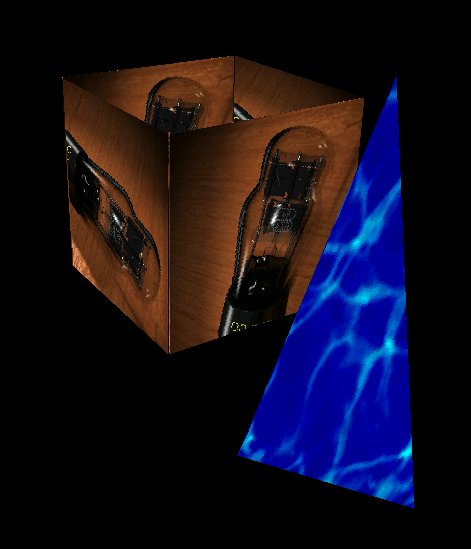
The design of three-dimensional objects is still an awkward process; NRDL provides help in this respect with its wrap family of functions. The idea is to wrap a texture around some basic geometrical figure. Currently implemented are cylinders and spheres, each of which can be double-layered or single-layered, solid or hollow, and complete in circumference or only partial. That is, the user can specify full spheres or only hemispheres, full cylinders or half-cylinders or any fraction of a cylinder, and so forth. Also implemented are rectangular prisms with the same options for single or double layer and simple flat planes (useful for describing the ground or the sky outdoors). Each family of shapes has a module specific to it, and any number of modules could be added: cones and pyramids, prisms with arbitrary tops and bottoms, etc.
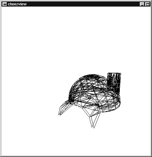
Another critically important design tool which was developed, and
an entire application on its own, was the simple wireframe previewer
Cheezview. Cheezview allows a designer to navigate in a simple manner
through the world he or she has created. The ability to translate
and rotate about in three dimensions allows inspection of the general
structure of the objects in a world. Also, movement is bound to the
timestep event, so that event systems can be tested.
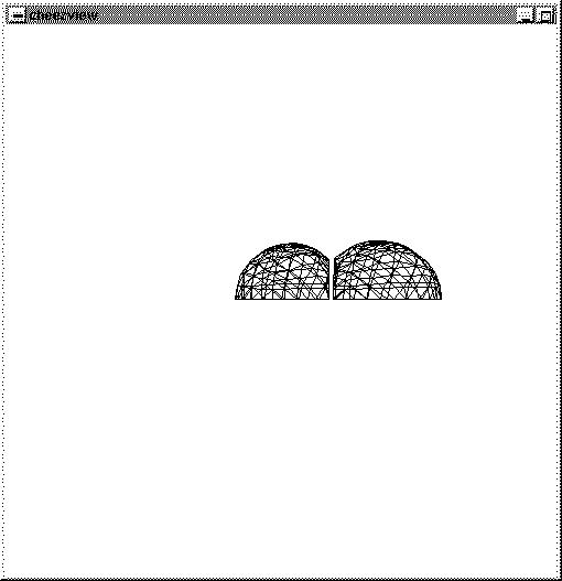
The latest and most interesting tool to be added to the NRDL suite is the structure-merging facility. This was developed as a solution to the problem of constructing large, complex objects by composing smaller ones when the desired effect is to have one continuous interior. For example, the user may wish to have a space made up of the interiors of intersecting spheres; there already existed procedures for simply composing the two spheres, but the desired effect is to also cut away the walls of the spheres where they intersect, creating a single uninterrupted volume.
The way to accomplish this effect is to choose a suitable dividing plane between the two structures, cut off the parts of either structure which stray within a specified distance of the plane, and connect the cut-off edges with a mesh of new triangles. A "suitable" dividing plane is one that causes the least number of original triangles to be lost. Still in development is an automated algorithm for determining the optimal dividing plane; at this moment the user must still specify the plane manually.
In a virtual world that is being rendered in real-time, speed is essential. The time that it takes to render a collection of polygons can be reduced significantly if you have an efficient way of determining which polygons are in front of other polygons from a particular point of view. Given that many virtual worlds are largely composed of static objects, it makes sense to spend a large amount of time prior to the rendering setting up a scene description which can be quickly traversed during the rendering step. BSP trees are particularly well suited to this task, given their efficiency and versatility.
Given N initial polygons, the construction of a BSP tree can take up to O(2^N) in the worst case, but in the expected case (which is significantly more likely) the running time is more like E(N^2) with a significant constant factor. Once the BSP tree is constructed, the time that it takes to determine the Z-order of every polygon from a particular point of view is O(N) with even better expected time performance when using culling techniques. The time that it takes to determine the Alpha Maps for every polygon in the scene also takes O(N) with a huge constant factor.
A BSP Tree is used to recursively divde up an n-dimensional space using (n-1)-dimensional hyperplanes. In the case of 3 dimensions this means that the space is divided up using planes, and in the case of 2 dimensions the space is divided using lines.
As can be seen from the following diagram, each division of the space introduces an additional node into the BSP tree.

In order to take advantage of the structure of a BSP tree, the dividing hyperplanes are chosen to completely contain individual polytopes of the scene, (in the case of 3 dimensions these are polygons, in the case of 2 dimensions they are line segments.) By containing a polytope within each hyperplane the scene can be completely divided using O(n) hyperplanes.
By using this particular data structure many things can be determined about the scene quickly and efficiently, such as the z-order of the polygons, or the visibility of particular light sources, as shall be explained later.
A BSP tree looks like a standard binary tree with a certain collection of information stored at each node of the tree: the paritioning plane that was used to divide the space at that node, the list of polygons that are contained internally within that partitioning plane, and two pointers to the current node's children.
BSP Node
Plane Paritioning_Plane
Polygon_List Internal
BSP_Node * Front
BSP_Node * Back
The list of static polygons is generated by the dynamically linked level library.
The compiler is responsible for creating a balanced BSP tree given a collection of polygons as input. It does this by recursively descending through the space, choosing partitioning planes and dividing the polygons as it goes along.
The compiler begins by iterating across the list of polygons that compose the scene. For each polygon, a temporary plane is created that completely contains that polygon. Using this plane, the compiler then determines the total number of polygons that lie on each side of the plane, the number of polygons that are intersected by the plane, and the number of polygons that are contained within the plane. Using these values, it is then possible to assign a particular score to that particular partitioning plane.
Score = abs [(# in front) - (# in back)] * BALANCE_IMPORTANCE + (# intersecting) * SPLIT_IMPORTANCE;
After assigning a particular score for each possible partitioning plane the compiler chooses the plane with the lowest possible score and partitions the space accordingly. All of the polygons that are contained by the plane are added to the Internal polygon list for that particular node of the BSP tree. All of the polygons in front are added to the Front-list, all the polygons in back are added to the Back-list, and all of the polygons that are intersected by the plane are split into front and back polygons and then added to the appropriate list.
After assigning all of the polygons to the appropriate lists, the compiler creates two new nodes, the front node and the back node. The compiler then recursively compiles these two nodes using the Front-list for the front node and the Back-list for the back node.
After the compiler has incorporated each polygon the job if finished.
An additional piece of information that is stored at each node of the BSP tree is an axis-aligned bounding box. This bounding box is the smallest possible box that will still contain all of the polygons that are internal to the node and all of the polygons which are contained within the node's children.
The bounding box for each node is computed in a bottom up fashion by computing the bounding box at the leaves of the tree and then computing the bounding box for each node of the tree based upon its internal polygon list and the bounding boxes of its children.
These bounding boxes will be amazingly useful for frustum culling and visibility determination, as shall be explained later.
Given a static scene with static lighting, it is possible to generate shadows and other lighting effects prior to real-time rendering. This is done by creating an Alpha Map for each polygon in the scene. An Alpha Map is a grid like assignment of intensity values to different portions of the polygon. These intensity values indicate the total amount of illumination that reaches each particular point on the polygon. During rendering, this Alpha Map will influence the final texture that is applied to the polygon and thus becomes visible at that point. Many effective and beautiful lighting techniques can be used in the creation of Alpha Maps since the total number of light sources only affects the time that it takes to preprocess the scene, not the time it takes to render it.
The Alpha Maps are created by iterating across each polygon in the BSP tree. For each polygon, an appropriately sized Alpha Map is created. (For large polygons a large Alpha Map is created, for a small polygon a smaller Map is used. The size of the Alpha Map indicates the granularity of the lighting effects. Larger Alpha Maps mean smoother lighting effects, but they also require significantly more memory.) For each grid point on the polygon the preprocessor determines the total amount of illumination that that point receives. This is done by iterating across each light source in the scene. For each light source, the preprocessor determines if the light source is visible from the view point of the grid point. This can be done using an O(n) traversal of the BSP tree. If the light source is visible, the illumination of the point is increased by:
Illumination += (Intensity of Light Source) / ((Distance to light source) ^ 2)
This technique generates smooth gradients, but shadows are still sharp edged. For a more accurate "area light source" effect, you can simply add more lights to the scene since this does not affect the time that it takes to render in real-time.
While rendering the scene, the scanline converter needs to receive polygons in back to front order. It is the duty of the BSP tree to provide that information, and given a particular viewer origin, it is a relatively simple matter to traverse the BSP tree and generate the back to front ordered list of polygons.
We begin at the root node. If the viewer's origin is in front of the partitioning plane for this node, then we want to draw all of the polygons that are behind the plane, then all of the polygons that are contained within the plane, and then all of the polygons that are in front of the plane. If the viewer is behind the plane then we simply do the same thing in reverse. If the viewer's origin is within the plane then the order of rendering does not matter since there is no way for polygons on either side to obstruct each other.
It is that easy.
We simply recurse through the tree in this fashion until every polygon has been drawn. This ultra-quick traversal method is one of the main beauties of BSP trees. One of the other beautiful qualities is the ease with which unnecessary polygons can be culled from the scene.
BackFace Culling is the removal of every polygon in the scene that is oriented away from the viewer's current location. This form of culling assumes that each polygon is one sided and has a normal that points in the direction of that side. By performing BackFace Culling it should be possible to remove most of the unnecessary polygons and cut the total number of polygons sent to the scanline converter roughly in half.
In order to do BackFace Culling efficiently an additional piece of information has to be stored for each polygon: the NormalAlignment. This value indicates whether or not the polygon in question is oriented in the same direction as the partitioning plane that contains it. This piece of information can be determined and stored during the compilation of the BSP tree.
Once we have this piece of information, it becomes a simple matter to perform BackFace Culling while traversing the BSP tree. If the viewer's line of sight is oriented with the normal of the partitioning plane, (the dot product of the two values is nonnegative,) then the plane is facing in the wrong direction and every polygon that has a normal oriented in the same direction as the plane should not be displayed, whereas all of the other polygons should be displayed. This selection process is reversed if the plane normal is *not* oriented with the viewer.
During real-time rendering of the scene, the viewer's origin will move around, the viewer's direction of sight will move, the viewer's up-vector (the amount of tilt) will move, even the field of view of the viewer could potentially change. An efficient description of all of this information is the viewer's frustum.
A frustum is the truncated pyramid that describes the total volume which is visible to the viewer. It has a top plane, a bottom plane, a right plane, a left plane, a back plane, a front plane, and an origin. While viewing the scene, there is no need to render any polygon that is not contained at least partially within the viewing frustum. This form of polygon removal is called frustum culling.
Given the hierarchical nature of the BSP tree and the bounding box information that it contains, it is an efficient matter to cull almost all polygons that do not lie within the frustum.
At each node of the tree we check to see if the bounding box of the node is completely outside or completely inside of the tree. If it is completely outside then we know that no part of the subtree will ever be visible and we can thus return without rendering any polygons. If it is completely inside then we know that every part of the subtree is visible and thus as we traverse the subtree there is no reason to check for Frustum visibility. If the bounding box is not completely outside or completely inside, then we have to run on the assumption that everything is visible and continue our tree traversal, making frustum visibility checks at each node along the way.
In addition, if the bounding box was not found to be completely inside, then we also need to check each polygon to see if it is within the viewing frustum. But, given the high cost of doing a complete determination, we instead simply look for trivial rejection, and otherwise assume that the polygon is in fact visible. It is possible for us to let a few polygons slip through that are beyond the X or Y reach of the frustum since the scanline converter can do X & Y clipping efficiently.
A more awkward problem though is the issue of a polygon that is partially within the frustum but whose face extends back behind the viewer. In this case, weird scanline effects can result due to the negative Z values generated. It is thus necessary to clip such polygons against the front plane of the frustum while traversing. This can be done relatively efficiently, but the real hope is that there will only be a small number of polygons that need to be clipped in such a manner.
There were many difficulties associated with building the BSP tree compiler and traverser, along with the light preprocessor. Many of these difficulties had to do with the mathematical trickiness of the calculations involved. Many more difficulties had to do with the sheer size and complexity of the code, (currently over 3000 lines.) And yet, all of these difficulties were overcome.
When it came time to integrate the BSP components with the other two components there were also a collection of difficulties in making the merger as smooth as possible. Certain types had to be extended to allow portability between the different modules. Certain scale and orientation assumptions had to be massaged. Several inconsistencies between C and C++ also had to be resolved. In general though, the modules were abstracted enough to allow relatively easy integration.
There are many other things that I would like to implement using this BSP framework.
One thing that I would like to try and explore is using different scoring techniques during compilation. I have noticed that certain types of scenes can cause very unbalanced BSP trees and I think I may have some solutions that will make the balancing step more efficient and intelligent. In particular I want to try and incorporate variants on the following values into my scoring technique.
(# contained) * INTERNAL_IMPORTANCE
(Ratio of total area of polygons contained vs.
total area of all polygons) * RATIO_IMPORTANCE
In addition, I also really want to try some intelligent portal/sector methods for determining visibilitiy culling. I have several ideas for how to implement the portals very efficiently and I am looking forward to playing around with them.
The scan converter is responsible for converting the abstract polygonal representation of the world into a viewable scene. This task involves more than just the drawing of triangles to a frame buffer; the scan converter must also manage textures, apply lighting effects, clip triangles that extend across the boundaries of the viewing window, transform the scene depending on the eye position and orientation, etc.
An absolute requirement for the scan converter is speed. By far the most time-consuming element of creating a real-time virtual environment is the final rasterization (as opposed to, say, object manipulations). Thus, it is imperative that the scan converter be as highly optimized as possible. To this end, much attention was paid to the quality of the assembly language code generated by the C compiler, and fixed-point integer arithmetic was used almost exclusively, to avoid the comparatively slow floating-point code generated by most compilers. Floating-point arithmetic will likely be included once the inner loops are hand-coded in assembly, since x86 processors can execute floating-point and integer operations in parallel.
I will describe the general principles of operation of my scan converter, to a moderate level of detail. I will not, however, describe some algorithms (like the structure of the innermost rendering loop), due to the potential usability of this engine in a commercial product. For the same reason, I have not included source code for the scan converter.
The rendering stage of the graphics pipeline receives a Z-ordered list of triangles from the BSP tree. This list has been roughly culled to the viewing frustum and also clipped to exclude any polygons exceedingly close to the eyepoint. The renderer translates the polygons to the eyepoint, then rotates them about the eyepoint. At this point the frustum's axis is the Z axis (extending in the positive direction to infinity), the eyepoint is the origin, and the viewing plane is parallel to the X-Y plane at some point on the positive Z axis. Finally, the renderer performs the perspective transformation to produce image-space coordinates.
The polygon list is passed to the scan converter. The current algorithm used is the painter's algorithm, in which all polygons are drawn in back-to-front order. Depending on future needs, this technique may be scrapped for a more efficient one.
A triangle taken from the list is drawn in two phases: the upper half and lower half. The halves are divided by whichever vertex lies in the middle between the uppermost and lowermost vertices. While the algorithm for filling these two half-triangles is the same, various parameters must be updated at the middle. Additionally, for triangles whose top two vertices lie on the same scanline, the first half-triangle fill must be skipped. The three vertices are sorted in top-to-bottom order.
Two counters, x1 and x2, are initialized to the X coordinate of the topmost vertex. Two deltas, dx1 and dx2, are computed for, respectively, the left and right edges of the upper half-triangle. Two other deltas, dx3 and dx4, are calculated for the lower half-triangle; one of them will be the same as dx1 or dx2. For each scanline, dx1 and dx2 are added to x1 and x2, tracing the two edges. When the middle vertex is reached, dx3 and dx4 are added to x1 and x2 instead.
Filling a scanline is the innermost loop of the scan converter. The line is traversed from x1 to x2 and each pixel is drawn to the frame buffer.
As mentioned earlier, the painter's algorithm is used, so the rearmost triangles are drawn first, to be overlaid later by closer triangles. Thus, there is no Z-buffer and no comparisons are performed during scanline traversal.
Special precautions must be taken if a triangle intersects the edge of the screen. For the right and bottom edges, the solution is simple: just stop drawing. However, for the left and top edges, the per-edge and per-line tracers must be primed with the appropriate values to correctly draw the clipped triangle. This is done primarily by adding multiples of the deltas by the amount of the triangle that is offscreen. Note that, unlike a generic triangle-to-rectangle clipping algorithm, this algorithm requires essentially zero extra processing to deal with any clipping situation, since the clipping occurs explicitly during scan-conversion, rather than symbolically at the polygon level.
Of course, the triangle filler described above has no particular source of data to place in the frame buffer. There are a multitude of different triangle patterning algorithms: flat shading, Gouraud shading, Phong shading, texture mapping, depth cueing, etc. Texture mapping is by far the most flexible, since it permits the application of realistic bitmaps to triangles, rather than the more abstract modifications of single colors (or interpolations of colors) of the other methods.
The most straightforward way to texture-map a triangle is to specify, for the triangle's three vertices, the X and Y values on a texture bitmap to appear at those vertices. For example, to map the upper left triangle of an arbitrary bitmap to some soon-to-be-texture-mapped triangle, we could specify that the three vertices of the new triangle correspond to coordinates (0,0), (99,0), and (0,99) on the source bitmap. Then, as we trace the triangle, we interpolate the X and Y texture values along the triangle's edges and across each scanline, fetching the correct pixel from the source bitmap as we traverse. This is done in a manner very similar to the dx method used to trace the triangle's edges, except that the interpolation must also be done across the scanline. Thus, there are eight variables, tx1, ty1, tx2, ty2, dtx1, dtx2, dty1 and dty2 that trace the texture along the triangle's edges, and four more, tx, ty, dtx and dty, that trace the texture along a given scanline.
This naive implementation of the texture-mapping algorithm produces strikingly effective results. After optimization, and with some restrictions on textures (such as the requirement that their dimensions be a power of two), the inner scan-conversion loop was thirteen x86 instructions. This gave a texture-mapping speed of on the order of 80,000 triangles per second on an AMD K6-233.
However, this algorithm does not take into account the perspective transformation. A perspective-correct texture mapping algorithm must reverse the perspective transformation at each pixel it fills in order to stretch the texture on portions of a triangle that are nearer to the viewer. We initially thought that the errors introduced by the naive algorithm would be noticeable but rather mild, but once we started feeding the scan converter scenes that were representative of the real applications of our engine, we found that perspective distortion was in fact horrendous. So it became obvious that perspective correction was essential.
When doing a straight Z-buffering algorithm, the easiest way to track Z as a polygon is scan-converted is to linearly interpolate 1/z (often called h) along the polygon's edges and scanlines. This correctly handles the nonlinear aspect of perspective. In order to apply this to the mapping of a texture, the scan converter tracks h across the polygon, just as for a Z-buffering algorithm. However, instead of using Z to determine polygon ordering, the difference between the current Z and the Z of the previously rendered pixel on the scanline is used, in conjunction with a precomputed scale factor, to determine how much to move across the texture for each one-pixel increment of the regular scan-converter.
As an initial test of this algorithm, it was implemented only in the code that traverses the edges of the polygon. The code for a single scan line was left untouched. This immediately fixed all of the perspective distortion seen earlier. There is undoubtedly still some distortion because the correction is not applied across the scanline. Perspective correction will be implemented across a scanline only if excessive distortion appears after further testing, or if it can be fit into the inner loop without undue slowdown.
Unfortunately, the simple addition of the per-line correction code also caused a substantial slowdown, and ways to speed this up are being actively researched.
One of the most striking advances that the game Quake made over its predecessor, Doom, was its use of static lighting. In Doom, areas were fairly uniformly lit, but in Quake, there are real light sources that create real gradients on walls, and objects cast real shadows. Because the lights are static, all of this lighting data can be precalculated. During rendering, maps of the light's contribution to a texture's brightness, the alpha maps, are applied to the textures. This saves immense amounts of memory, both in RAM and on disk, since every modified texture need not be saved, and since an alpha map can be of a different (presumably lower) resolution than the texture.
We are currently integrating alpha maps into our renderer. Initially, these alpha maps will be implemented right alongside the texture mapper, within the inner loop of the scan converter. A later version will likely apply the alpha maps to the rendered scene once the entire scene is rendered and visible textures have been determined. This way, the number of alpha map applications can be reduced to only those textures that are known to be visible.
For ease of coding, speed, power and flexibility, nothing beats the Linux operating system as a development environment. The system was written to run on a Linux machine with a recent version of the XFree86 X server running in 16 bit mode. The scan-conversion code is profoundly non-portable, as it makes many assumptions about the x86 processor, its data types and its instruction set, and the code also requires the DGA feature of XFree86. When DGA is enabled, the X server returns a pointer to the start of video memory, and the user process is free to write directly to that RAM without the intervention of the X server. This is the fastest, most straightforward (and non-portable) way to get colors to the screen.
The test machine was an AMD K6-233 with 64 MB of FPM RAM and 1 MB of synchronous pipelined burst cache SRAM, and a Matrox Mystique PCI video card with 4 MB of RAM. The video card was run at 1600x1200 resolution, with 16 bits of color. The K6-233 is actually running at 225 MHz, but the bus speed of the system was overclocked to 75 MHz from its normal 66 MHz to increase PCI bus speeds to 37.5 MHz, increasing maximum theoretical throughput to the video card from 133 MB/sec to 150 MB/sec. This can make a noticeable difference in rendering speed. (The screen resolution also makes a minor difference in rendering speed; this is presumably because the video memory bandwidth needed to refresh a frame on the CRT is significantly higher at 1600x1200 than, say, at 640x480, leaving less free time for the renderer to write to video RAM.)
The initial plan for the scan converter was to use spanning scan-line algorithm, with the world represented by an unordered list of polygons. It was assumed that we would come up with an efficient way of eliminating polygons, and that the spanning scan-line angorithm would efficiently deal with Z ordering, but a trial implementation was terribly slow. One of the advantages of this method, though, is that it allows the entire world to be dynamic - since there is no BSP tree, the tree does not have to be reordered if and when triangles move around. However, the outstanding efficiency of the BSP tree, coupled with the ease of optimization of a scan converter whose sole purpose is to draw a triangle as fast as possible, soon made it obvious that we needed to go with our current plan.
I am taking 6.111 this term, and my final project is a hardware 3D accelerator. If my partner and I manage to make it work, it should be fairly simple to take the output of Colin's BSP tree and send it directly to my hardware, which draws triangles (not texture mapped, yet...) at the rate of 20 megapixels per second.